Detecting Rare Earth Elements

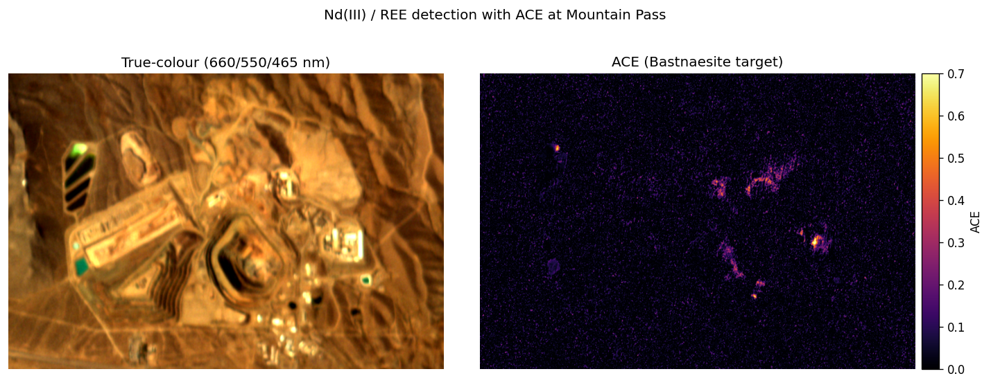
The goal of this tutorial: an Nd detection map (right) built from a Wyvern scene over the Mountain Pass REE mine (left).

Try it yourselfRuns free in your browser with no install or setup, and pulls the imagery straight from our Open Data Program.Or view the notebook source on GitHub

Open in Colab

Rare earth elements (REEs) power everything from electric vehicles to wind turbines, and finding new sources is a strategic priority. It turns out several REEs leave a spectral fingerprint we can see from orbit. Neodymium (Nd) in particular produces sharp, characteristic absorption features in the visible / near-infrared (VNIR) at roughly 585, 745, 810 and 870 nm, and — crucially — those positions barely move regardless of the host mineral. That makes Nd a reliable proxy for REE-bearing material.

This tutorial is inspired by a great paper: Asadzadeh, Koellner & Chabrillat (2024), Detecting rare earth elements using EnMAP hyperspectral satellite data: a case study from Mountain Pass, California. It reports the first direct detection of Nd from a spaceborne hyperspectral satellite (earlier REE mapping had been done from the lab, the ground, and aircraft, but not from orbit). This tutorial will create an approachable and easy to run workflow in three small steps:

1. Continuum removal to isolate the absorption features from overall brightness.
2. Spectral resampling of a real USGS bastnaesite reference spectrum onto Wyvern's bands.
3. ACE (Adaptive Cosine Estimator), a matched-filter-style detector, to map Nd-bearing pixels.

Use L2A surface reflectance

REE absorptions are subtle. This workflow needs L2A surface reflectance (atmospherically corrected) imagery. If you run it on L1B top-of-atmosphere radiance, the solar spectrum and the oxygen absorption band near 760 nm will swamp the features. All imagery on the Open Data Program is L2A unless otherwise noted.

Getting started

The companion notebook is self-contained and installs its own dependencies, so there is nothing to set up in advance.

• Google Colab (easiest): open the notebook using the "Open in Colab" badge at the top of it, then run the cells top to bottom.
• Local Jupyter: open the notebook in JupyterLab or VS Code (Python 3.10+) and run it.

Either way, the first cell installs the packages that are not already present:

%pip install -q rasterio spectral scipy pyarrow

The image we're using

We use a Wyvern Dragonette-002 scene over Mountain Pass, California, available as an L2A surface-reflectance product on the Wyvern Open Data Program. The notebook downloads it automatically from its STAC item.

The Nd fingerprint

Neodymium in its common +3 oxidation state (Nd(III)) has a set of narrow absorption bands whose centre wavelengths barely shift with the host mineral, which is what makes them such a dependable fingerprint. Four fall within Wyvern's Extended VNIR range:

Feature	Wavelength	Notes
Nd 585 nm	~585 nm	Weaker, sits on the green-red slope
Nd 745 nm	~745 nm	Strong and diagnostic
Nd 810 nm	~800-810 nm	Strong; the true minimum is near 800 nm
Nd 870 nm	~870 nm	At the edge of the Extended VNIR range

Where the reference spectrum comes from

To recognize this fingerprint we need a known example to compare against. We use a laboratory spectrum of bastnaesite (the Nd-bearing carbonate mineral mined at Mountain Pass) from the USGS splib07 spectral library, the standard, freely available reference library of minerals and materials measured under controlled laboratory conditions.

Rather than parsing the USGS library's native format, we access it through OpenSpecLib v0.0.6, an open-source project that repackages the splib07 release (a large collection of per-spectrum ASCII data files, alongside the ECOSTRESS and ECOSIS spectral libraries) as Apache Parquet files. That means we can pull a single reference spectrum with a couple of lines of pandas, with no special readers required; we simply download the pre-built Parquet file straight from the OpenSpecLib release rather than installing anything. We use the bastnaesite entry splib07a_Bastnaesite_REE_WS320_crystl_ASDFRb_AREF; the library also contains pure neodymium oxide and other REE minerals (monazite, samarium oxide, and more) if you want to experiment.

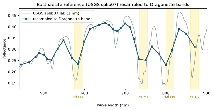
The USGS splib07 bastnaesite reference at full 1 nm resolution (grey) and resampled to Dragonette's bands (blue); we'll cover the resampling in the "Resample a real reference spectrum" section below. Note the Nd features at the shaded windows.

Code

Imports and configuration

import io

import requests
import numpy as np
import pandas as pd
import rasterio
from rasterio.warp import transform_bounds
from rasterio.windows import from_bounds
from scipy import ndimage
from spectral.algorithms.detectors import ace as spy_ace
import matplotlib.pyplot as plt

# Wyvern Open Data Program STAC item (L2A surface reflectance) for the Mountain Pass scene.
STAC_ITEM = (
    "https://wyvern-odp.com/application/mining/"
    "wyvern_dragonette-002_20250422T221452_2bc40137_l2a/"
    "wyvern_dragonette-002_20250422T221452_2bc40137_l2a.json"
)
REFLECTANCE_SCALE = 1e-4  # L2A scaled integers -> 0..1 reflectance

# The ODP item is the full satellite swath, so we crop to a bounding box around the
# Mountain Pass mine (min_lon, min_lat, max_lon, max_lat, WGS84) before analysis.
AOI_BOUNDS = (-115.555, 35.470, -115.515, 35.492)

# Pre-built Parquet asset published with the OpenSpecLib release; we download it
# directly for convenience instead of installing openspeclib and converting splib07 ourselves.
OPENSPECLIB_PARQUET_URL = (
    "https://github.com/null-jones/openspeclib/releases/download/v0.0.6/usgs_splib07.parquet"
)
BASTNAESITE_ID = "usgs_splib07:splib07a_Bastnaesite_REE_WS320_crystl_ASDFRb_AREF"

ND_FEATURES = [585, 745, 810, 870]  # diagnostic Nd(III) VNIR features, nm

After downloading the scene from the Open Data Program (see the notebook for the STAC download helper), we read the band centre wavelengths and per-band FWHM (Full Width at Half Maximum) straight from the GeoTIFF. Because the ODP item is the full swath, we reproject the AOI to the image CRS and crop to our AOI, then scale to reflectance:

def read_wavelengths_and_fwhm(dataset: rasterio.DatasetReader) -> tuple[np.ndarray, np.ndarray]:
    """Read band centre wavelengths and FWHM (both in nm) from a Wyvern GeoTIFF.

    Args:
        dataset: An open rasterio dataset for a Wyvern GeoTIFF.

    Returns:
        A tuple of the band centre wavelengths and the band FWHM values, both in nm.
    """
    centres, fwhm = [], []
    for band in range(1, dataset.count + 1):
        centres.append(float(dataset.descriptions[band - 1].split("_")[1]))
        fwhm.append(float(dataset.tags(band)["FWHM"]))
    return np.asarray(centres), np.asarray(fwhm)


with rasterio.open(local_file) as src:
    wavelengths, fwhm = read_wavelengths_and_fwhm(src)
    # Reproject the AOI to the image CRS and read only that window.
    left, bottom, right, top = transform_bounds("EPSG:4326", src.crs, *AOI_BOUNDS)
    window = from_bounds(left, bottom, right, top, src.transform)
    window = window.round_offsets().round_lengths()
    cube = src.read(window=window).astype("float32")
    cube[cube == src.nodata] = np.nan
    profile = src.profile
    profile.update(
        height=cube.shape[1],
        width=cube.shape[2],
        transform=src.window_transform(window),
    )

cube *= REFLECTANCE_SCALE

Continuum removal

An absorption feature is easiest to measure relative to the local spectral background, or "continuum". We divide each pixel's spectrum by its upper convex hull, so absorptions show up as dips below 1.

This is the classic continuum-removal method of Clark & Roush (1984), Reflectance spectroscopy: Quantitative analysis techniques for remote sensing applications (J. Geophys. Res. 89, 6329-6340). The continuum is the convex hull fitted over the top of the spectrum, representing the background reflectance if the absorption were absent; dividing the spectrum by that hull normalizes the features to a common baseline so their depths and positions can be compared between pixels and against library spectra. The same technique underpins USGS Tetracorder and the continuum removal tools in ENVI and the EnMAP-Box.

def continuum_removed(wavelengths: np.ndarray, reflectance: np.ndarray) -> np.ndarray:
    """Continuum-remove a spectrum by dividing by its upper convex hull.

    Args:
        wavelengths: Band centre wavelengths in nm.
        reflectance: Reflectance values at those wavelengths.

    Returns:
        The continuum-removed spectrum (1.0 is on the continuum, lower is absorption).
    """
    points = list(zip(wavelengths, reflectance))
    hull: list[tuple[float, float]] = []
    for p in points:
        while len(hull) >= 2:
            (x1, y1), (x2, y2) = hull[-2], hull[-1]
            if (x2 - x1) * (p[1] - y1) - (y2 - y1) * (p[0] - x1) >= 0:
                hull.pop()
            else:
                break
        hull.append(p)
    hull_x = [h[0] for h in hull]
    hull_y = [h[1] for h in hull]
    return reflectance / np.interp(wavelengths, hull_x, hull_y)

Plotting a pixel over the ore-handling area, before and after continuum removal, the Nd dips pop out at the shaded feature windows:

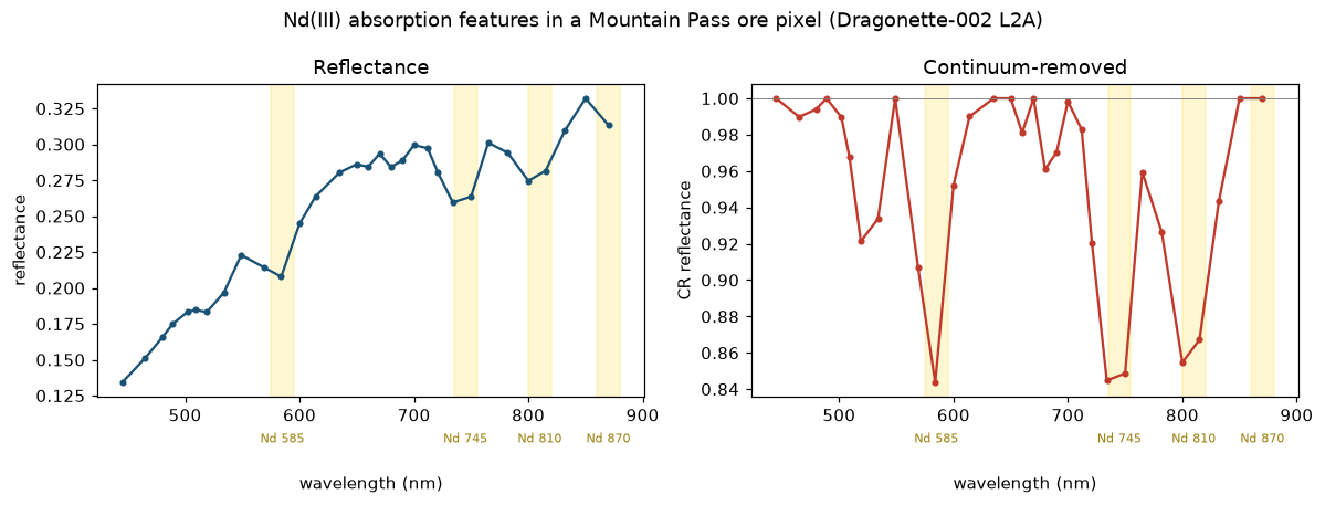
A Mountain Pass ore pixel. After continuum removal the Nd absorptions at 585, 745 and 810 nm are clear.

Notice the 810 nm dip reads a little shallow, because Dragonette's 815 nm band sits slightly off the true ~800 nm minimum. This matters less for the full-spectrum ACE detector below: it matches the shape of the whole spectrum at once, so no single band's depth decides the result.

Resample a real reference spectrum

Rather than hand-pick band positions, we compare each pixel to a real laboratory spectrum of bastnaesite (the Mountain Pass ore mineral) from the USGS splib07 library, packaged in OpenSpecLib v0.0.6. We resample it onto Wyvern's bands by convolving with each band's response (a Gaussian approximated from the FWHM), so the reference is blurred to the same spectral resolution as the imagery.

def load_reference(parquet_url: str, reference_id: str) -> tuple[np.ndarray, np.ndarray]:
    """Load one USGS splib07 spectrum from an OpenSpecLib parquet file.

    Args:
        parquet_url: URL of the usgs_splib07.parquet OpenSpecLib release asset.
        reference_id: The id of the spectrum to load.

    Returns:
        A tuple of wavelengths in nm and reflectance (0..1), with bad bands set to NaN.
    """
    raw = requests.get(parquet_url, timeout=600).content
    df = pd.read_parquet(io.BytesIO(raw), columns=["id", "spectral_data.values"])
    values = np.asarray(
        df.loc[df["id"] == reference_id, "spectral_data.values"].iloc[0], dtype="float64"
    )
    values[(values < 0) | (values > 1.5)] = np.nan  # USGS bad-band flags
    # splib07a wavelength grid: 2151 samples, 350-2500 nm at 1 nm spacing
    # (measured on an ASD field spectroradiometer).
    wl_nm = np.linspace(0.34999999, 2.5, 2151) * 1000.0
    return wl_nm, values


def resample_to_bands(
    ref_wl: np.ndarray, ref_refl: np.ndarray, centres: np.ndarray, fwhm: np.ndarray
) -> np.ndarray:
    """Convolve a fine reference spectrum onto sensor bands using Gaussian responses.

    Args:
        ref_wl: Reference wavelengths in nm.
        ref_refl: Reference reflectance at those wavelengths.
        centres: Sensor band centre wavelengths in nm.
        fwhm: Sensor band FWHM in nm.

    Returns:
        The reference reflectance resampled to the sensor bands.

    Note:
        For simplicity this approximates each band's response as a Gaussian derived
        from its FWHM. A rigorous workflow would instead convolve with each band's
        actual relative spectral response (RSR) curve, which is published for
        Dragonette in the Wyvern public resources:
        https://github.com/Nrevyw/wyvern-public-resources/tree/main/relative-spectral-responses
    """
    good = np.isfinite(ref_refl)
    wl, refl = ref_wl[good], ref_refl[good]
    out = np.empty(len(centres))
    for i, (centre, width) in enumerate(zip(centres, fwhm)):
        # Gaussian approximation of the band response (see Note; real RSR curves
        # would be more faithful).
        weight = np.exp(-0.5 * ((wl - centre) / (width / 2.3548)) ** 2)
        out[i] = np.sum(weight * refl) / np.sum(weight)
    return out


ref_wl, ref_refl = load_reference(OPENSPECLIB_PARQUET_URL, BASTNAESITE_ID)
target = resample_to_bands(ref_wl, ref_refl, wavelengths, fwhm)

The USGS bastnaesite reference at full 1 nm resolution (grey) and resampled to Dragonette's bands (blue).

Detect with ACE

The Adaptive Cosine Estimator (ACE) scores how well each pixel aligns with the reference direction after the scene background has been statistically "whitened" (mean-subtracted and decorrelated using the scene covariance). ACE is insensitive to overall brightness, which makes it a robust, easy-to-threshold detector. ACE is bounded between 0 and 1 where values closer to 1 are stronger matches to the reference spectra.

For a pixel spectrum $x$, target $t$, scene mean $m$ and covariance $C$, with centred vectors $\tilde{x} = x - m$ and $\tilde{t} = t - m$, the score is:

$$\mathrm{ACE}(x) = \frac{\left(\tilde{t}^{\top} C^{-1} \tilde{x}\right)^2} {\left(\tilde{t}^{\top} C^{-1} \tilde{t}\right)\left(\tilde{x}^{\top} C^{-1} \tilde{x}\right)}$$

Intuitively, $C^{-1}$ whitens the background so common, high-variance materials do not dominate, and the expression is the squared cosine of the angle between the whitened pixel and the whitened target.

We use the ACE implementation in Spectral Python (SPy), a common hyperspectral package, and wrap it only to drop nodata pixels and reshape the result. Because we cropped to the mine, the scene is small, so this is fast and light.

def detect_ace(cube: np.ndarray, target: np.ndarray) -> np.ndarray:
    """Adaptive Cosine Estimator detection score over a reflectance cube.

    The detection is delegated to Spectral Python's ace; we only drop nodata
    pixels and reshape the result back onto the image grid.

    Args:
        cube: Reflectance cube (bands, rows, cols) with nodata set to NaN.
        target: Target reflectance vector (length equal to the number of bands).

    Returns:
        A 2D array of ACE scores in 0..1, with NaN where the cube is invalid.
    """
    bands, rows, cols = cube.shape
    flat = cube.reshape(bands, -1).T
    valid = np.isfinite(flat).all(axis=1)
    out = np.full(flat.shape[0], np.nan, dtype="float32")
    out[valid] = spy_ace(flat[valid], target)
    return out.reshape(rows, cols)


ace = detect_ace(cube, target)

Mapping the ACE score next to a true-colour view, the strongest matches land squarely on the mine's ore-handling and stockpile areas:

ACE detection score (right). Bright pixels are the strongest matches to the bastnaesite reference.

Overlay the detections on the RGB preview

A detection map is most useful laid over a familiar view. We threshold the ACE score, apply a little morphological cleanup to drop isolated single-pixel hits and thicken the rest for visibility, then blend the result over the true-colour composite.

DETECTION_THRESHOLD = 0.2

mask = np.nan_to_num(ace) > DETECTION_THRESHOLD
# Additional processing: remove isolated single-pixel hits, then thicken slightly.
mask = ndimage.binary_opening(mask, structure=np.ones((2, 2)))
mask = ndimage.binary_dilation(mask, iterations=1)

rgb = stretch(660, 550, 465)
fig, ax = plt.subplots(figsize=(9, 7))
ax.imshow(rgb)
overlay = np.where(mask, ace, np.nan)
im = ax.imshow(
    overlay, cmap="turbo", vmin=DETECTION_THRESHOLD, vmax=np.nanmax(ace), alpha=0.9
)
ax.set(title=f"Nd(III) detections (ACE > {DETECTION_THRESHOLD}) over RGB")
ax.axis("off")
fig.colorbar(im, ax=ax, fraction=0.046, pad=0.02, label="ACE")
plt.tight_layout()
plt.show()

The 0.2 threshold is an empirical choice based on this scene's score distribution, not a magic number: background ACE scores cluster near zero (the scene median is ~0.01 and even the 99th percentile is ~0.18), so a 0.2 cutoff keeps only the extreme tail of strongest matches, which top out near 0.79. If you adapt this workflow to another scene or target, inspect the ACE histogram and tune the threshold to balance missed detections against false positives.

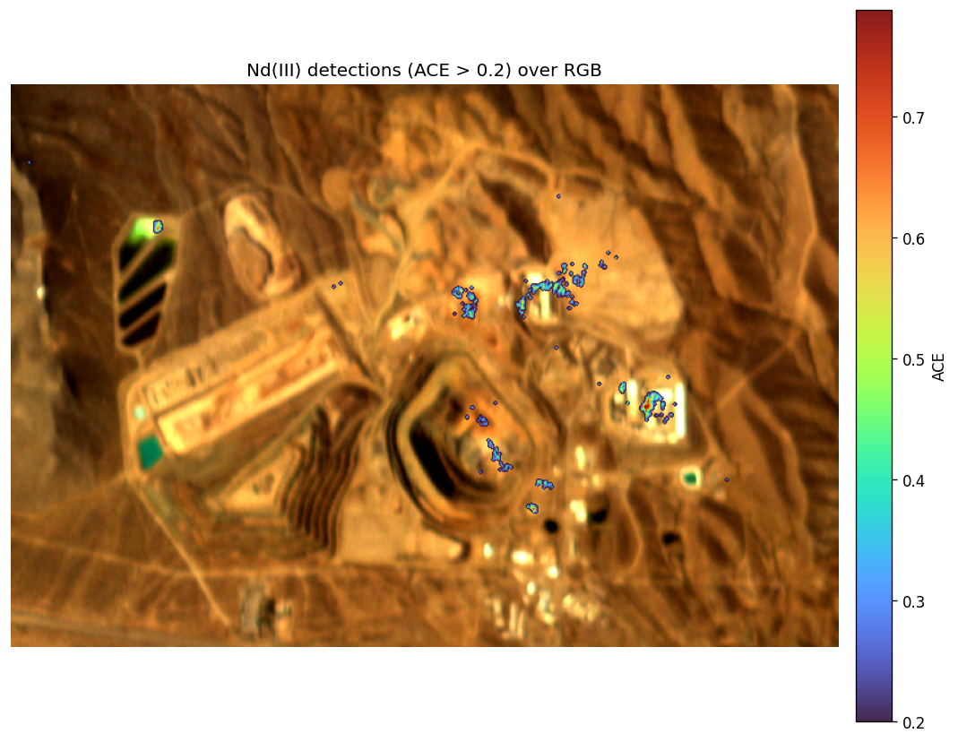
Cleaned Nd(III) detections (ACE > 0.2) blended over the true-colour composite, concentrated on the ore-handling and stockpile areas.

Always sanity-check

A detector is only trustworthy if the pixels it flags actually look like the target. Overlaying the continuum-removed spectra of the top-scoring pixels against the reference, they share the same Nd absorptions, confirming the detection is real, not an artifact:

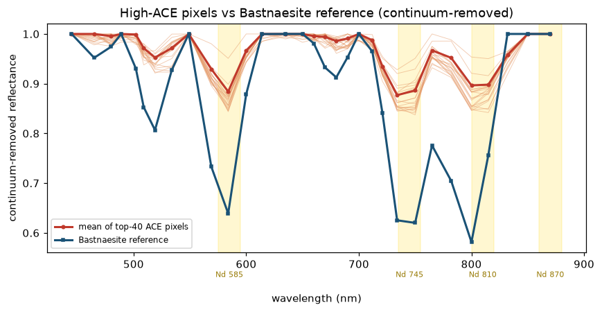
Top-scoring pixels (orange, red = mean) reproduce the Nd absorptions of the bastnaesite reference (blue).

Wrap-up

You continuum-removed a Wyvern spectrum, resampled a real USGS bastnaesite reference to Dragonette's bands, and used ACE to map Nd-bearing material at Mountain Pass, reproducing, in miniature, the idea behind the EnMAP study.

A few things to keep in mind:

• It is an exploration, not proof of REE. Treat detections as candidates to follow up, and always sanity-check their spectra.
• Spectral resolution matters. Dragonette's ~20-30 nm bands broaden the narrow Nd features, so measured depths are smaller than a lab or a finer-resolution sensor would see. Comparing against a full reference spectrum (as ACE does) is what keeps the detection robust.

Want to go further? Try the pure neodymium-oxide reference instead of bastnaesite, threshold the ACE map to export candidate polygons, or explore other detection methods like Spectral Angle Mapper and Mixture Tuned Matched Filtering. Share what you build on our GitHub Discussions!