Loading & Viewing Wyvern Data in Python

Output color infrared image from the Python notebook

Try it yourselfRuns free in your browser with no install or setup, and pulls the imagery straight from our Open Data Program.Or view the notebook source on GitHub

Open in Colab

Note: There are many ways to visualize raster data using Python. The combination of Rasterio + Matplotlib was chosen due to the simplicity & ability to build off of this code.

Getting started

• Google Colab (easiest): open the notebook using the "Open in Colab" badge above, then run the cells top to bottom.
• Local Jupyter: open the notebook in JupyterLab or VS Code (Python 3.10+) and run it.

Either way, the first cell installs the packages that are not already present:

%pip install -q numpy matplotlib requests rasterio

Image we're using

Check out the image on the Wyvern Open Data Catalog!

This is L2A surface reflectance data, meaning atmospheric effects have already been corrected for and pixel values represent an estimate of actual ground reflectance rather than raw at-sensor radiance.

Band Combinations

We'll be exploring the following band combinations!

Name	Red Channel	Green Channel	Blue Channel
Natural Color (RGB)	650nm	550nm	503nm
Color Infrared (CIR)	750nm	650nm	550nm

Code

First things first, let's import all of our packages.

import json
import numpy as np
import rasterio
import matplotlib.pyplot as plt

Download the Tutorial Files

Let's download the GeoTIFF and its STAC JSON metadata!

Run the cell below to download these files. Once the download is complete, they'll appear in the same folder as your notebook!

import requests
from pathlib import Path

IMAGE_URL = "https://wyvern-data.com/wyvern_dragonette-001_20240930T070744_08fd7f5a_l2a/wyvern_dragonette-001_20240930T070744_08fd7f5a_l2a.tiff"
JSON_URL  = "https://wyvern-odp.com/wyvern_dragonette-001_20240930T070744_08fd7f5a_l2a/wyvern_dragonette-001_20240930T070744_08fd7f5a_l2a.json"

IMAGE_PATH = Path("wyvern_dragonette-001_20240930T070744_08fd7f5a_l2a.tiff")
JSON_PATH  = Path("wyvern_dragonette-001_20240930T070744_08fd7f5a_l2a.json")

downloads = [
    (IMAGE_URL, IMAGE_PATH),
    (JSON_URL, JSON_PATH),
]

for url, path in downloads:
    if path.exists():
        print(f"{path.name} File already here! Skipping download.")
    else:
        print(f"Downloading {path.name}...")
        response = requests.get(url, headers={"User-Agent": "Mozilla/5.0"})
        response.raise_for_status()
        path.write_bytes(response.content)

print("Downloads complete!")

Loading the Data

We'll start by reading the scale factor from the metadata JSON file we downloaded earlier. Wyvern's L2A products represent surface reflectance, but the values are stored as scaled 16-bit integers to reduce file size.

# Open the JSON metadata file and extract the scale factor
with open(JSON_PATH) as json_file:
    metadata = json.load(json_file)

# The scale factor converts stored uint16 reflectance values into their floating-point representation
scale_factor = metadata["assets"]["Cloud optimized GeoTiff"]["raster:bands"][0]["scale"]

# if you don't have the JSON file, you can hardcode the scale factor:
# scale_factor = 0.0001

print(f"Scale factor: {scale_factor}")

Now let's open the GeoTIFF using rasterio. We'll replace any nodata pixels with np.nan so they are excluded from our calculations, then apply the scale factor to recover the floating-point reflectance values.

with rasterio.open(IMAGE_PATH) as image_file:
    # Convert to float so we can use np.nan and decimal values
    image_arr = image_file.read().astype(np.float32)
    nodata = image_file.nodata
    band_descriptions = image_file.descriptions

# Replace nodata pixels with NaN so they are excluded from calculations
if nodata is not None:
    image_arr[image_arr == nodata] = np.nan

# Apply the scale factor to recover floating-point reflectance values
image_arr *= scale_factor

print(f"Image shape: {image_arr.shape}")
print(f"Image bands: {', '.join(band_descriptions)}")

Building the Wavelength Map

Unlike a standard RGB image, each band in a hyperspectral GeoTIFF corresponds to a specific wavelength. We can find this information in the eo:bands field under the GeoTIFF asset in the STAC JSON we downloaded earlier, which lists each band's center wavelength. We'll read these out and build a map from wavelength to band index so we can select bands by wavelength rather than hardcoding band numbers.

with open(JSON_PATH) as json_file:
    metadata = json.load(json_file)

wavelength_map = {}
for i, band in enumerate(metadata["assets"]["Cloud optimized GeoTiff"]["eo:bands"]):
    wavelength = round(band["center_wavelength"] * 1000)  # convert from μm to nm
    wavelength_map[wavelength] = i

print(wavelength_map)

Selecting Bands by Wavelength

Now we'll write a small helper function that finds the nearest available band to any wavelength we ask for. This means if we request 550nm and the closest available band is 549nm, it'll find it automatically.

def get_band(wavelength_nm: int) -> np.ndarray:
    """
    Returns the image band closest to the requested wavelength.

    Args:
        wavelength_nm: Target wavelength in nanometres.

    Returns:
        A 2D array containing reflectance values for the closest available wavelength band.
    """
    available_wavelengths = list(wavelength_map.keys())
    closest_wavelength = min(available_wavelengths, key=lambda w: abs(w - wavelength_nm))
    print(f"Requested {wavelength_nm}nm -- using {closest_wavelength}nm")
    return image_arr[wavelength_map[closest_wavelength]]

Now that we have the image array loaded, we're good to plot it using matplotlib!

# Select our R, G, and B bands by wavelength, then stack them into a [rows, columns, channels]
# array which matplotlib expects
rgb_arr = np.dstack([get_band(650), get_band(550), get_band(503)]).astype(np.float32)

brightness_factor = 3  # Bring up the brightness a touch so we have a better visual
rgb_arr_bright = rgb_arr * brightness_factor
rgb_arr_bright = np.clip(rgb_arr_bright, 0, 1)  # keep values within 0-1

# We specify a larger figsize to get a better resolution out of the image. You can
# increase this further to further improve resolution! (at the expense of file size)
fig, ax = plt.subplots(1, 1, figsize=(15, 10))
ax.imshow(rgb_arr_bright)

plt.tight_layout()
plt.show()

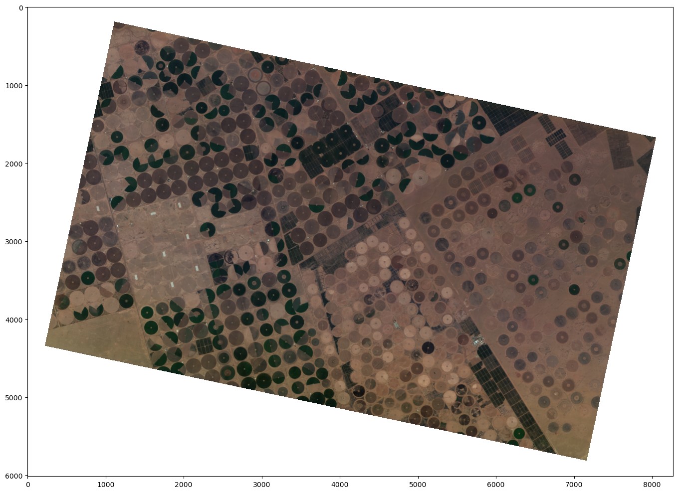
Output true-color image from the Python notebook

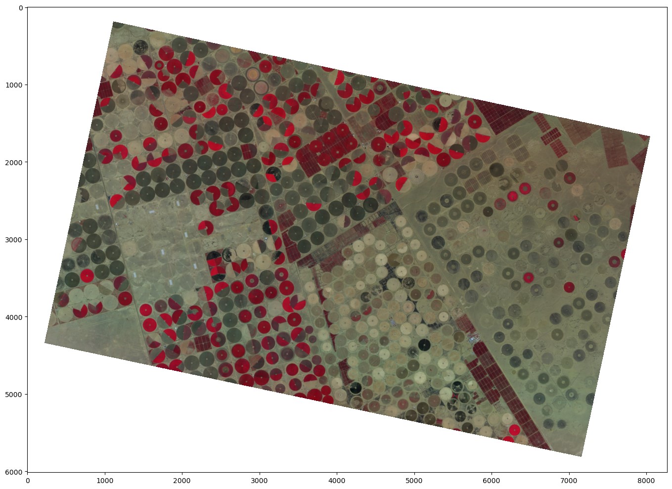
We can also render the image in color infrared by selecting a different set of bands from the image.

# Now, let's do the same with color infrared!
cir_arr = np.dstack([get_band(750), get_band(650), get_band(550)]).astype(np.float32)

cir_arr_bright = cir_arr * brightness_factor
cir_arr_bright = np.clip(cir_arr_bright, 0, 1)  # keep values within 0-1

fig, ax = plt.subplots(1, 1, figsize=(15, 10))
ax.imshow(cir_arr_bright)

plt.tight_layout()
plt.show()

Output color infrared image from the Python notebook

Well done! You now know how to download and view Wyvern images in Python! Jump to the next tutorial to make some super cool plots about hyperspectral pixels!