Using Dragonette Imagery Data In ENVI Software

Introduction

The purpose of this tutorial is to provide a quick high-level introduction to some of the different ways in which Wyvern's satellite imagery data products acquired by their Dragonette satellites can be utilized in the ENVI® desktop software application while highlighting a handful of real-world analysis use cases. Rather than an exhaustive walkthrough, this tutorial covers some of the most popular basic functionality available in the ENVI software that is compatible with Wyvern's imagery products, including data ingest, preprocessing, interactive analysis, and automated algorithms for hyperspectral data exploitation. Finally, Wyvern does not explicitly endorse any specific commercial software tools and cannot provide technical assistance on the utilization of the ENVI software, if you have any specific questions on the ENVI software please contact your NV5 technical support representative.

ENVI® Software Overview

The ENVI® geospatial analysis software is developed, distributed, maintained, and supported by NV5 Geospatial. It is an industry standard image processing and geospatial data analysis application used by image analysts and data scientists around the world to extract timely, reliable, and accurate information from remote sensing imagery. The focus of this tutorial is on the modern ENVI v5+ desktop software interface and this tutorial does not cover the legacy ENVI Classic application.

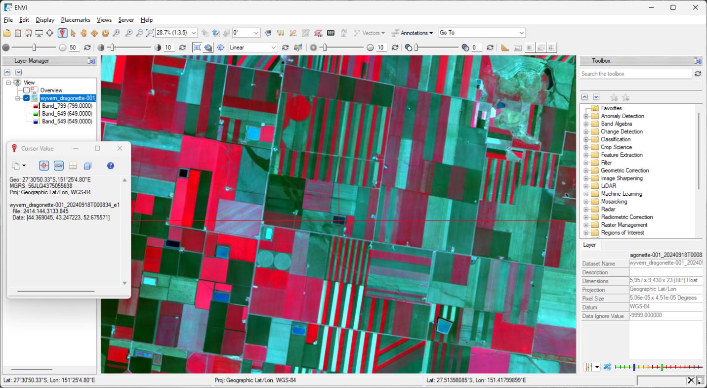
Figure 1 – Wyvern Dragonette-1 imagery data product loaded into the ENVI software (CIR)

ENVI is a leader in spectral image processing and analysis, with top tools for multi and hyperspectral data including spectral target detection and identification. These tools are based on established, scientific methods for spectral analysis, using pixel responses at different wavelengths to obtain information about the materials within each pixel. They are used to detect objects, map features, measure vegetation health, identify minerals, detect marine debris, measure pollution, analyze wildlife habitats, map oil slicks, evaluate water quality, mitigate wildfires, detect methane leaks, perform supervised land use land cover (LULC) classification, and provide novel intelligence insights for numerous peace & security use case applications.

Data Ingest & Display

The first step when working with Dragonette imagery products is to ingest the raster dataset into the ENVI desktop software. The ENVI software has built-in smart data ingest readers which have intelligent support for a wide variety of Raster Formats including Wyvern's Dragonette imagery data products. The optimal method for opening Wyvern imagery data products will depend on the version of ENVI desktop software that is being utilized.

ENVI v6.0 (or older)

In order to open the Wyvern imagery data product into the ENVI desktop software application use the File -> Open… menu option then select the imagery data product raster TIFF file or drag-n-drop this *.tiff file onto the ENVI display window. While the TIFF file format has band center wavelengths metadata embedded into the *.tiff file which are ingested by ENVI there is not currently a dedicated TIFF tag for storing wavelength units which are important to assign to the raster dataset in order to unlock certain downstream ENVI software functionality. Consequently, the recommended process of opening a Wyvern imagery dataset into ENVI v6.0 (or older) software is the following multi-step process:

1. File -> Open… menu option then select the imagery data product raster TIFF file (or drag-n-drop this *.tiff file onto the ENVI display window).
2. In the Layer Manager panel on left-hand side of ENVI application either double-click on the wyvern_dragonette-* image layer or right-click on the layer and in the resulting context menu select View Metadata.
3. At the bottom-right corner of the resulting View Metadata pop-up window press the Edit Metadata button.
4. At the upper-left corner of the resulting Edit ENVI Header pop-up window press the + Add… button.
5. In the resulting Add Metadata Items pop-up window scroll down in the list and select Wavelength Units then press the OK button to dismiss the dialog.
6. Back in the Edit ENVI Header dialog navigate to the Spectral tab and make sure the Wavelength Units field drop-down list is set to Nanometers then press OK button with the Display Result box checked (on) which will reload the image into the display window.

ENVI v6.1 (or newer)

In order to open the Wyvern imagery data product into the ENVI desktop software application use the File -> Open As -> Optical Sensors -> Wyvern menu option then select the STAC metadata JSON file (in the same subfolder next to the TIFF image file) or drag-n-drop this *.json metadata file onto the ENVI display window. While using the menu option File -> Open… or drag-n-drop opening of the TIFF image file will still work in the ENVI v6.1 (or newer) application the dedicated Wyvern raster data ingest method using the JSON metadata file provides enhanced downstream ENVI software functionality. Consequently, the recommended process of opening a Wyvern imagery dataset into ENVI v6.1 (or newer) software is a much simpler single-step process:

1. File -> Open As -> Optical Sensors -> Wyvern menu option then select the STAC metadata JSON file (or drag-n-drop this *.json file onto the ENVI display window).
2. In the Layer Manager panel on left-hand side of ENVI application either double-click on the wyvern_dragonette-* image layer or right-click on the layer and in the resulting context menu select View Metadata.

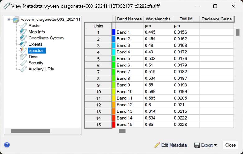
Figure 2 – Raster metadata information for a Wyvern Dragonette Level-1B imagery dataset

Color Band Combinations

By default when a Wyvern Dragonette imagery data product is opened into the ENVI software it will automatically display a True Color (RGB) band combination image rendering of the raster dataset in the main display window at 100% (1:1) resolution positioned at the center of the image scene. A detailed overview of how to use the ENVI software user interface and the display window navigation controls (Pan, Zoom, Rotate, Go To, etc.) is beyond the scope of this tutorial so for more information on the ENVI user interface basics please refer to NV5's online documentation for the ENVI software Display Tools.

In order to generate the RGB true color image display the ENVI software will automatically select the spectral bands with center wavelengths closest to the Red, Green, and Blue portions of the visible electromagnetic spectrum. Furthermore, the ENVI software has other Dynamic Band Selection controls that are easily customized via the panel in the lower-right hand corner of the main ENVI user interface (which is available at the bottom of the Layer tab whenever a raster is the selected layer in the Layer Manager). Since Dragonette imagery data has spectral bands that cover the visible and near-infrared (VNIR) wavelengths there are two predefined color band combinations that work well with Wyvern datasets: True Color (RGB) and Color Infrared (CIR). Furthermore, users can customize the image display band combination via click-and-drag of the individual blue & green & red slider bars in order to interactively select the bands for each color channel.

1. Click on the wyvern_dragonette-* image layer in the Layer Manager panel to make sure it is the selected active layer.

2. In the lower-right hand corner of the ENVI application window a Layer tab will be displayed that contains useful properties of the Dragonette imagery raster dataset.

3. At the bottom of this Layer tab panel click the dropdown arrow button to change the image display between True Color or Color Infrared predefined color band combinations in the resulting pop-up menu and observe how the image rendering is updated in the main display window. Experiment with other band combinations by moving the Blue & Green & Red tick marks on the color slider: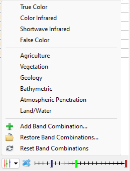

   

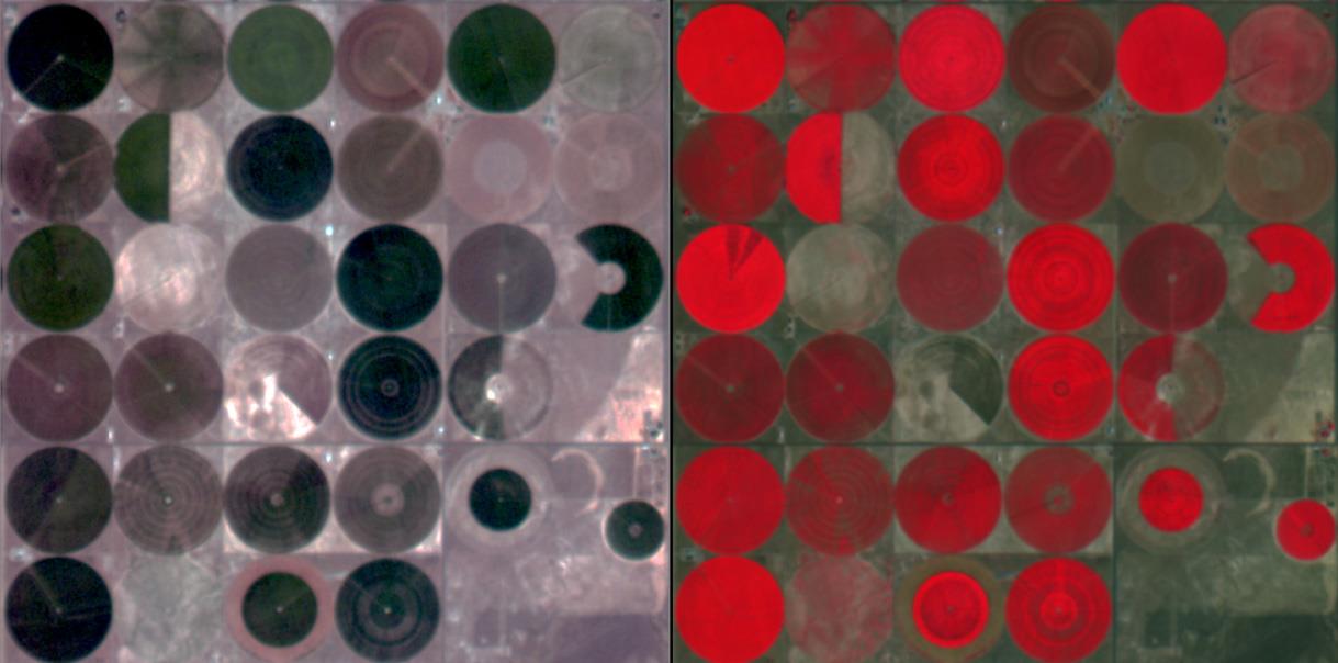
Figure 3 – Comparison of True Color (RGB) and Color Infrared (CIR) band combinations

Stretch Types & Stretch Extents

By default, the ENVI software will automatically display imagery datasets with a default Stretch Type, and for Wyvern imagery with a 32-bit floating-point (float32) pixel data type the Linear 2% quick stretch type will be applied. While the Linear 2% stretch should provide a reasonable initial image visualization it is best suited to the mid-range pixels, since it maximizes contrast by saturating the lowest 2% of pixels to all black and the highest 2% to all white while stretching the mid-range pixel values in between. Consequently, in order to effectively visualize features in the darkest and brightest range of pixels while still maintaining visual separation of nuanced pixel radiance intensity differences end users may benefit from selection of alternative stretch types and/or the stretch on extent options available in the ENVI software.

1. Open a Wyvern Dragonette imagery data product and display a color band combination image into the view window. By default, the ENVI software will display the image with a stretch type of Linear 2% which will be the selection in the stretch type drop-down list:

   

2. On the main toolbar at the top of the ENVI software window click on the stretch type drop-down list and experiment by selecting other stretch types. In particular, the Optimized Linear stretch type will avoid the saturation of low and high pixel intensities at the tail ends of the image histogram thereby retaining visual fidelity in the darker and brighter regions of the imagery: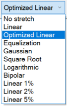

   

3. To the left of the stretch type drop-down list are three buttons that control the imagery area extent that is used to calculate the statistics for the current image stretch applied in the view display window. By default, the button will be selected for the Stretch on Full Extent mode which means the image stretch is based on statistics calculated on the data histogram of pixel values from the entire full extent of the imagery dataset.

4. In order to optimize the display stretch for the portion of the image currently displayed in the view window experiment with the other two stretch extent options:

   1. Press the button to select Stretch on View Extent mode which updates the image stretch for the current view extent a single time
   2. Press the button to select Stretch on View Extent with Auto Update mode which continuously updates the image stretch based on the current view extent while Pan & Zoom & Rotate movement occurs

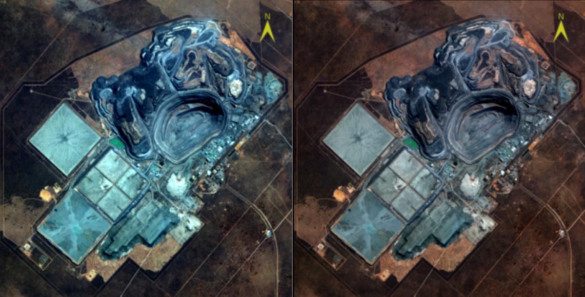
Figure 4 – Image with Optimized Linear stretch type (left) and stretch on view extent (right)

Brightness & Contrast & Sharpen

Once the desired image display stretch type and stretch extent has been selected the ENVI software also includes additional visual Enhancement Tools which can be applied by leveraging the brightness, contrast and sharpen sliders on the main toolbar at the top of the ENVI software window. All three of these image display enhancements can be used to improve the visual appearance of the imagery rendering within the active view window.

1. Start by selecting the Linear option from the stretch type drop-down list.
2. Locate the Brightness slider and drag the tick marker to a brightness value of 65. This will slightly increase the overall brightness of the current image display.
3. Locate the Contrast slider and drag the tick marker to a contrast value of 0. This will eliminate any extra contrast enhancement in order to display the original imagery.
4. Locate the Sharpen slider and drag the tick marker to a sharpen value of 100. This will apply the maximum sharpening which will enhance the edges of smaller features within the imagery.

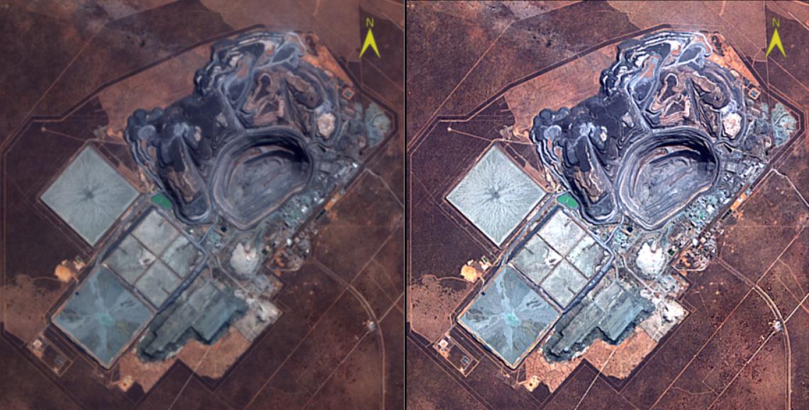
Figure 5 – Image display with no Contrast (left) and increased Brightness & Sharpen (right)

Statistical Analysis

The ENVI software provides a wide variety of statistical analysis techniques for imagery raster datasets that can quickly & easily identify anomalous image pixels or segregate spectrally distinct regions.

RX Anomaly Detection

The ENVI software includes a simple RX Anomaly Detection tool that runs the Reed-Xiaoli Detector (RXD) algorithm which identifies pixels that are spectrally distinct from the overall imagery dataset background and thus represent anomalies within the image scene. In order for the RXD algorithm to be effective the anomalous targets must be relatively small in comparison to the overall spatial extent of the image scene. Results from the RXD analysis tool are unambiguous and have proven highly effective in detecting subtle spectral features within any given hyperspectral imagery dataset. The output raster generated by the RXD algorithm can also highlight anomalous scan lines but these do not affect the detection of other valid spectrally anomalous pixels within the image scene.

1. Within the Toolbox panel on the right-hand side of the ENVI software window type rx string in the blank search text box, press the Enter key on the keyboard, and double-click on the resulting RX Anomaly Detection tool that is highlighted.
2. Make sure to select the Wyvern Dragonette imagery dataset as the Input Raster, set the Suppress Vegetation parameter to the appropriate setting depending on whether vegetation should be considered anomalous by the RXD algorithm, then specify an output raster filename.
3. Press the OK button to run the RXD algorithm and the resulting output anomaly raster dataset will be generated then displayed as a single-band grayscale image with higher pixel values representing more spectrally anomalous pixels.
4. Within the Toolbox panel reset the search and enter band roi string in the blank search text box, press the Enter key, and double-click on the resulting Band Threshold to ROI tool that is highlighted.
5. In the resulting Choose Threshold dialog click-n-drag the maximum line on the anomaly raster histogram plot then move the maximum line all the way to the right-hand side of the plot window to set the Max Value for the region-of-interest (ROI) as the maximum RXD raster dataset pixel value.
6. Set the Min Value for the ROI by typing a minimum anomalous pixel intensity value of 20 in the text box then press the Enter key on the keyboard.
7. Once the band threshold ROI is generated in the Data Manager pop-up window right-click on the New ROIs item in the list and select Load.

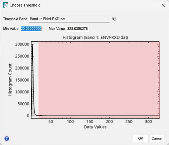
Figure 6 – Band threshold to ROI dialog with selection of high anomaly detection pixels

The resulting ROI that was generated by thresholding the highest anomalous pixel values from the RXD algorithm output raster will be displayed as bright red color on top of the current active view image display.

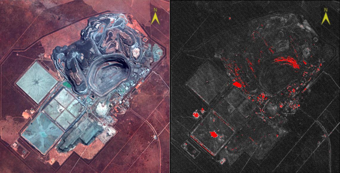
Figure 7 – RGB color image (left) and red anomaly pixels identified by RXD algorithm (right)

2D Scatter Plot

The ENVI software includes a convenient 2D Scatter Plot visualization tool that plots the pixel intensity values from one spectral band versus another spectral band which helps illustrate the degree of correlation between the two bands. It also provides a variety of interactive data exploration capabilities. For example, the scatter plot tool provides the ability to interactively view the distribution of pixel values within a patch moved under the cursor by clicking on the image display (called 'dancing pixels') along with region-of-interest drawing capabilities within the scatter plot in order to perform a simple supervised classification of the hyperspectral dataset.

1. With an imagery dataset displayed and selected in the Layer Manager panel select Display -> 2D Scatter Plot from the main menu or press the button on the toolbar at the top of the main ENVI software user interface window.
2. Experiment with the interactive band selection sliders available next to the X (horizontal) and Y (vertical) axes in order to select different spectral bands for the scatter plot visualization. Note that if the same band is selected for both X and Y the resulting scatter plot will be a simple linear line with a uniform slope since the same band is perfectly correlated with itself.
3. Setup the scatter plot tool visualization with a selection of the green wavelength Band 0.535 µm for the X axis band and infrared wavelength Band 0.799 µm for the Y axis band.
4. From the Scatter Plot Tool dialog menu select Options -> Patch Size -> 25 in order to increase the pixel patch size for the interactive dancing pixels visualization.
5. Back on the main ENVI software window click-n-drag within the active view display window to move the pixel patch box around in the image then see the corresponding dancing pixels highlighted in bright red color within the 2D scatter plot window.
6. Within the Scatter Plot Tool dialog window click-and-drag to interactively draw a polygon around an isolated section of the scatter plot pixels in order to define region-of-interest (ROI) class. In order to classify unique distinct features in the imagery dataset draw ROI class polygons around the separate isolated clusters of pixels in the scatter plot.
7. Repeat the process of drawing separate distinct ROI polygons for multiple separate classes by pressing the button to create a new class then draw a corresponding polygon within the scatter plot and note that any given pixel in the scatter plot can only belong to one individual ROI class.

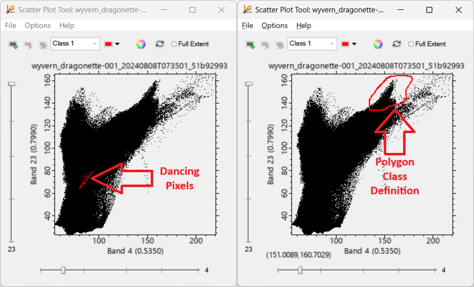
Figure 8 – 2D scatter plots with dancing pixels (left) and interactive class definition (right)

By creating multiple separate region-of-interest (ROI) classes in the 2D scatter plot dialog a simple supervised classification is effectively generated with each class color displayed on top of the source imagery dataset. These ROIs can also be used in subsequent supervised classification algorithms and processing workflows such as the Classification Workflow available in the toolbox panel on the right-hand side of the ENVI software window.

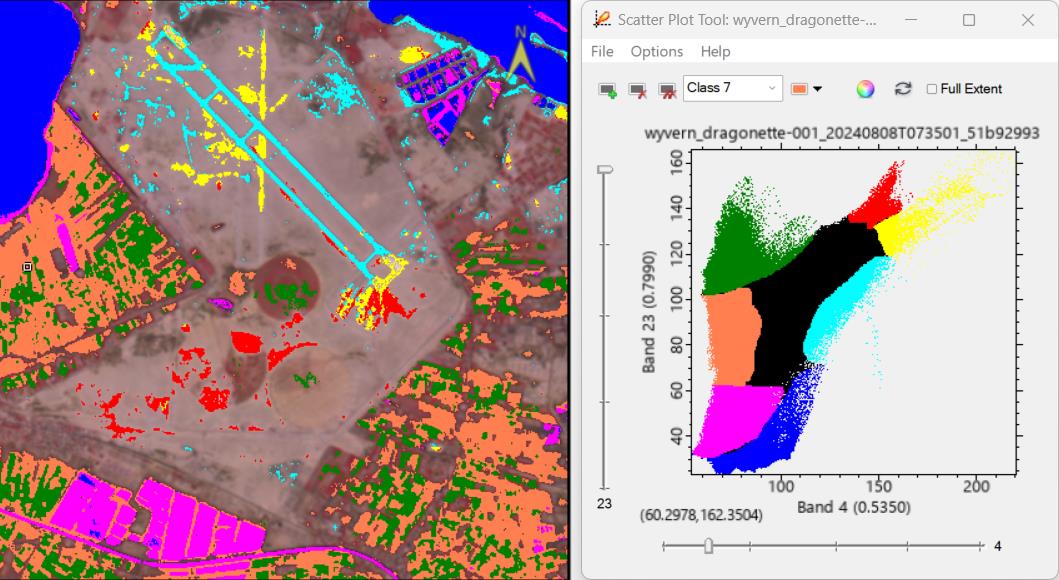
Figure 9 – Multiple region-of-interest (ROI) classes defined using the 2D scatter plot tool

ICA Transformation

The ENVI software includes the Independent Component Analysis (ICA) transformation algorithm which highlights the spectrally distinct features in the hyperspectral imagery data by amplifying the signal and suppressing the noise. The independent component analysis (ICA) algorithm decomposes data into independent signals and is a powerful processing technique for hyperspectral data in order to unmix the statistical independent endmembers. The ICA transformation can distinguish features of interest even when they occupy only a small portion of the pixels in the image.

1. Within the Toolbox panel on the right-hand side of the ENVI software window type forward ica new string in the blank search text box, press the Enter key on the keyboard, and double-click on the Forward ICA Rotation New Statistics and Rotate tool.
2. Select a Wyvern Dragonette hyperspectral imagery dataset in the resulting Independent Components Input File dialog then press the OK button.
3. Leave all ICA algorithm options configured with their default settings and specify an output ICA transformation raster dataset filename by pressing the Choose button to the right of the Enter Output Filename label.
4. Press the OK button to run the ICA algorithm and the resulting output ICA transformation raster dataset will be generated.
5. Display the ICA output raster dataset as RGB color using the lowest three bands which represent the most spectrally distinct and statistically independent data components of the input hyperspectral imagery dataset.

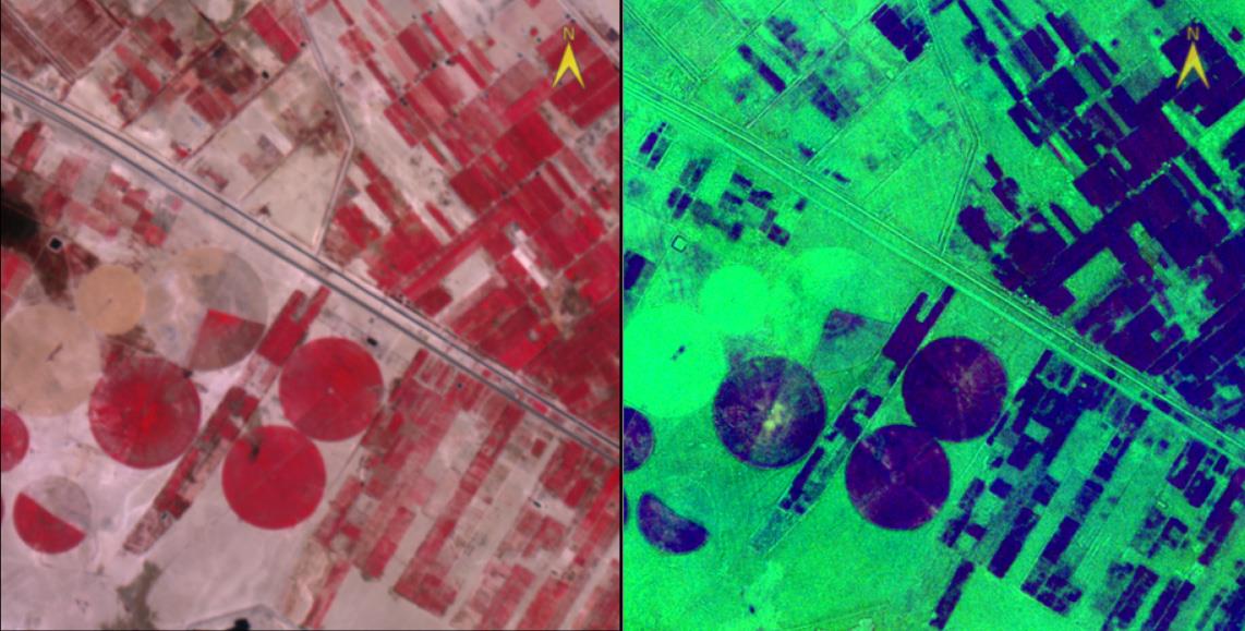
Figure 10 – The first three bands of ICA transformation displayed as RGB color image (right)

Atmospheric Correction

Wyvern's Dragonette imagery data products delivered with Level-1B (L1B) processing level have been radiometrically corrected to pixel units of at-sensor top-of-atmosphere (TOA) radiance based on spacecraft location plus pointing along with solar conditions at time of data acquisition. Since the L1B imagery data product is delivered as a raster dataset with 32-bit floating-point (float32) data type where the pixels represent top-of-atmosphere (TOA) radiance the imagery data is already in units of W / (m² * sr * µm) with no need to apply any scaling factor. Consequently, the L1B imagery data product can be immediately visualized and directly analyzed using the statistical analysis techniques described in the previous sections of this tutorial.

However, since the L1B imagery dataset's pixel values represent the solar illumination intensity as recorded by the hyperspectral imaging sensor on the Dragonette satellite in space the image data includes the impact of gases and aerosols in the atmosphere. In other words, the sunlight radiation has passed through the atmosphere twice before the final solar illumination intensity is recorded by the hyperspectral imaging sensor. Consequently, if the goal is analysis of the materials on the surface of the Earth a common pre-processing workflow is to first apply an atmospheric compensation correction to the L1B imagery product in order to remove the impact of atmospheric gases & aerosols thereby converting the image raster dataset pixels from top-of-atmosphere (TOA) radiance units to bottom-of-atmosphere (BOA) surface reflectance units.

Fortunately, the ENVI software has a dedicated Atmospheric Correction Module (ACM) with several atmospheric compensation modeling tools for this conversion. The atmospheric correction algorithms available in the ENVI software model the amount of gases, water vapor, and aerosols in the atmosphere based on the input source hyperspectral imagery dataset and other known metadata parameters such as the geographic location, acquisition time, solar elevation angle, etc. The computed atmospheric properties are then used to constrain highly accurate models of radiation transfer in order to remove the effects of the atmosphere and generate a new output raster imagery dataset where the pixel values represent an accurate estimate of the true surface reflectance at the bottom-of-atmosphere (BOA).

QUick Atmospheric Correction (QUAC)

One of the most powerful atmospheric compensation modeling algorithms available in the ENVI software for pre-processing of Wyvern's Level-1B (L1B) imagery data product is the QUick Atmospheric Correction (QUAC) tool. The ENVI software QUAC tool provides atmospheric correction of Wyvern's hyperspectral imagery datasets with spectral coverage across the visible and near-infrared (VNIR) wavelengths. QUAC determines the atmospheric correction parameters directly from the observed pixel spectra in an image scene without the need for the end-user to manually input additional ancillary information. QUAC is based on the empirical finding that the average reflectance of diverse material spectra is not dependent on each scene so processing is much faster compared to first-principles atmospheric modeling methods. QUAC allows for any imaging off-nadir angle or solar elevation angle and QUAC works best when there are multiple diverse materials in an image scene with sufficiently dark pixels to allow for a good estimation of the baseline spectrum.

1. Within the Toolbox panel on the right-hand side of the ENVI software window type quac string in the blank search text box, press the Enter key on the keyboard, and double-click on the QUAC - Quick Atmospheric Correction tool.
2. Select a Wyvern Dragonette imagery dataset and press the OK button.
3. In the resulting QUAC - Quick Atmospheric Correction dialog window make sure the Sensor Type drop-down list is set to Generic / Unknown Sensor which is the appropriate selection for Wyvern Dragonette imagery datasets.
4. Specify an Output Raster dataset filename and press the OK button to run QUAC.

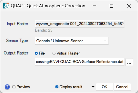
Figure 11 – Configuration of the QUAC - Quick Atmospheric Correction processing tool

Spectral Analysis

The ENVI software provides a wide variety of simple spectral analysis techniques for exploitation of hyperspectral imagery datasets. For the most accurate analysis of the materials on the surface of the Earth, the Wyvern L1B imagery data product should first be atmospherically corrected as described in the previous Atmospheric Correction section.

Spectral Profiles

The ENVI software provides a wide variety of interactive data plotting visualization tools where a common way to analyze hyperspectral imagery datasets is to extract spectral profiles (also known as Z profiles since they plot data values in the Z spectral dimension of a raster hypercube dataset). The Spectral Profile (Z Profile) tool in the ENVI software plots the pixel intensity spectrum for all spectral bands for any given pixel selected by the end-user clicking on selected image layers within the current active view window. ENVI uses the imagery product metadata and any custom header information to automatically scale and label the spectral profile plot. If multiple layers are displayed in the active view ENVI plots a Spectral Profile from each layer, to turn off the plot for an individual layer simply disable the check box for that layer in the Layer Manager.

1. With an imagery dataset displayed and selected in the Layer Manager panel select Display -> Profiles -> Spectral from the main menu or press the button on the toolbar at the top of the main ENVI software user interface window.
2. Make sure the ENVI software navigation controls are in active Select mode by selecting the button on the top toolbar or press the F5 key on the keyboard.
3. Using the mouse single-click on different pixels within the image display view window and the corresponding spectrum will be plotted as a line within the Spectral Profile dialog. The resulting spectral profile line plot represents the intensity of raster data values for the selected pixel throughout all of the spectral bands in the hyperspectral imagery data cube.
4. In order to analyze how the spectral signatures vary within the image scene use the mouse to click-n-drag across the image display view window then watch how the spectral profile line plot dynamically updates.
5. In order to collect multiple spectral profiles for different pixels within the image hold down the Shift key on the keyboard then use the mouse to left-click repeatedly within the image display view window on different areas of interest within the image scene and the corresponding spectral profile will be plotted for each pixel clicked.
6. On the right-hand side of the Spectral Profile dialog press the > bar button to expand the plot properties panel in order to see the list of collected spectra for the multiple pixels and select the Plot Stats tab to see useful data statistics for each pixel spectrum.

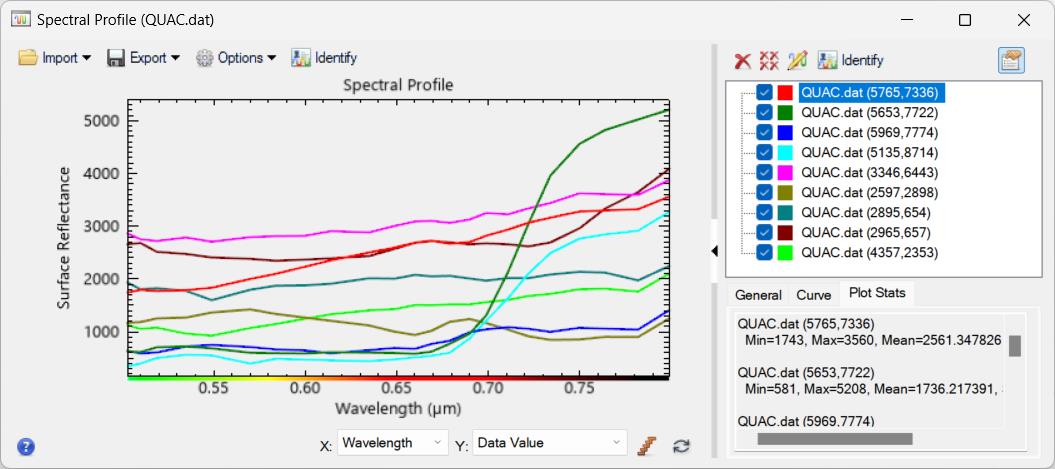
Figure 12 – Multiple spectral profiles generated with useful statistics for each pixel spectrum

The spectral profile plotting tool also provides a convenient way to visualize and inspect raster data pixel values from multiple imagery datasets in order to compare their respective spectral signatures. For example, an original Wyvern Level-1B (L1B) imagery dataset with top-of-atmosphere (TOA) radiance pixel units can be compared with the atmospherically compensated output result from the QUick Atmospheric Correction (QUAC) tool described in the previous section which generates a new imagery dataset with bottom-of-atmosphere (BOA) surface reflectance pixel units.

1. From the main ENVI software menu select Views -> Two Vertical Views or press Ctrl+2 on the keyboard.
2. Using the instructions in the ENVI software documentation for Multiple Views load the original Wyvern L1B imagery dataset into the first (left) view window then load the QUAC output imagery dataset into the second (right) view window.
3. From the main ENVI software menu select Views -> Link Views then in the resulting Link Views dialog select the Geo Link radio button option, press the Link All button, then press OK button to link the views and dismiss the dialog. This will ensure the two views are geographically linked so that each view displays the same location and extent of imagery.
4. Within the Layer Manager panel on left-hand side of ENVI software window select the original Wyvern L1B imagery dataset raster layer then press the button on the main toolbar in order to launch a new Spectral Profile plot for this dataset.
5. Within the Layer Manager panel on left-hand side of ENVI software window select the QUAC output result imagery dataset raster layer then press the button on the main toolbar in order to launch a new Spectral Profile plot for this dataset.
6. Make sure the ENVI software navigation controls are in active Select mode by selecting the button on the top toolbar or press the F5 key on the keyboard.
7. To compare spectral signatures from both imagery datasets use the mouse then click-n-drag across one of the image display view windows then watch how the spectral profile line plots dynamically update. This spectral profile comparison also illustrates how the Level-1B imagery dataset's slightly lower pixel intensity values in the 764 nm center wavelength band due to sunlight transmission impedance caused by oxygen absorption in the atmosphere has been corrected in the QUAC tool processing result output raster imagery dataset with surface reflectance units.

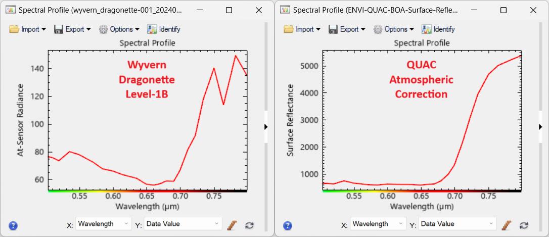
Figure 13 – Spectral profile comparison of original Wyvern Level-1B TOA radiance data (left) and the QUAC atmospheric correction output with BOA surface reflectance data (right)

Material Identification

The ENVI software includes a wide variety of advanced spectral analysis tools that can be used to extract useful insights from Wyvern's Dragonette hyperspectral imagery data products. One such capability is the Material Identification Tool, which compares any given imagery dataset pixel's unknown spectral profile against the spectra of known materials in ENVI's rich collection of reference Spectral Libraries, then ranks the similarity between the two using common spectral similarity algorithms. The tool can be found in the expanded plot properties panel on the right-hand side of any given Spectral Profile plot dialog window.

1. Open and display the QUAC atmospheric correction output processing result raster dataset so the imagery data being analyzed has bottom-of-atmosphere (BOA) surface reflectance pixel units.
2. Launch a new Spectral Profile for the QUAC-processed imagery dataset by selecting Display -> Profiles -> Spectral from the main menu or press the button on the toolbar at the top of the main ENVI software user interface window.
3. On the right-hand side of the Spectral Profile dialog press the > right arrow bar to expand the plot properties panel then press the button labeled Identify in order to launch the Material Identification tool.
4. Press the Select Library drop-down list button and select an appropriate spectral library *.sli file based on the potential materials contained in the imagery dataset. For example, the usgs_v7 -> vegetation_aviris.sli spectral library contains signatures for common vegetation materials derived from AVIRIS hyperspectral data which covers the same visible and near-infrared (VNIR) wavelengths as Wyvern Dragonette imagery datasets so it makes an excellent reference library for vegetative material identification.
5. Using the mouse single-click on the image display window to select a specific target pixel of interest then note how the Material Identification tool displays a top-down sorted table of potential spectral matches from the selected reference library.

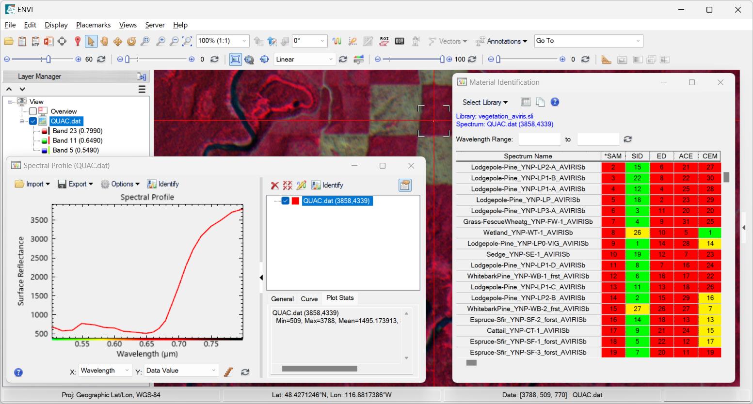
Figure 14 – Material identification based on USGS v7 spectral library showing high likelihood that selected imagery dataset pixel matches spectral signatures for Lodgepole Pine tree.

Spectral Indices

Since Wyvern's hyperspectral imagery datasets contain dozens of contiguous spectral bands with narrow bandwidths across visible and near-infrared (VNIR) wavelengths a very common and extremely powerful analysis technique is the extraction of Spectral Indices by applying specific predefined band algebra equations. The remote sensing science community has defined numerous spectral indices which leverage specific algebraic equations for band math arithmetic in order to highlight different features and properties within an Earth observation imagery dataset. Spectral indices are combinations of spectral reflectance from two or more wavelengths that indicate the relative abundance of features of interest such as fire burn severity, geologic minerals, man-made objects, built-up features, water & snow, soil & mud, and a wide variety of advanced vegetation properties. The ENVI software includes a convenient analytics tool for generating almost a hundred different spectral indices as delineated in the Alphabetical List of Spectral Indices including several specialized Narrowband Greenness vegetation indices which are specifically designed for advanced vegetative analysis of hyperspectral imagery datasets.

1. Open and display the QUAC atmospheric correction output processing result raster dataset so the imagery data being analyzed has bottom-of-atmosphere (BOA) surface reflectance pixel units.

2. Within the Toolbox panel on the right-hand side of the ENVI software window type indices string in the blank search text box, press the Enter key on the keyboard, and double-click on the Spectral Indices tool.

3. Select the QUAC output raster dataset and press OK button.

4. In the resulting Spectral Indices dialog window select the desired indices in the Index list in order to generate the new index raster(s) from the atmospherically corrected imagery dataset: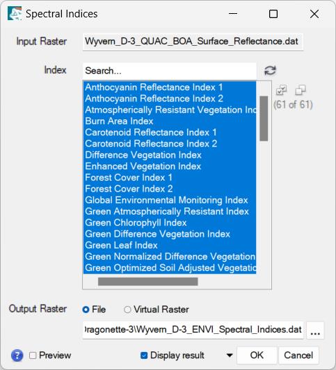

   

5. Once the spectral indices processing task is finished running open the Data Manager dialog, right-click on a spectral index band in the resulting output raster dataset, and select Load Grayscale.

6. Within the Layer Manager panel on left-hand side of ENVI software right-click on the spectral index raster layer, select Change Color Table -> More…, then within the Change Color Table dialog press the button to select a different color table.

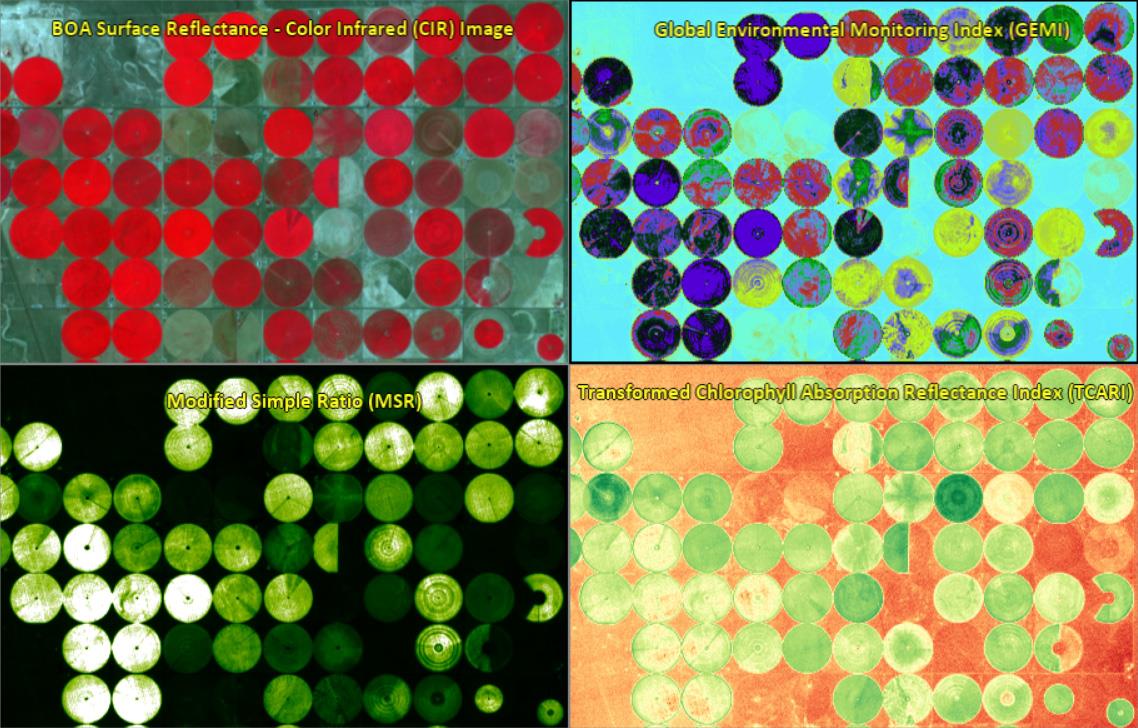
Figure 15 – Display of several spectral indices with different color tables applied

Advanced Analysis

Target Detection

Since the ENVI software includes a rich collection of several spectral libraries that contain the spectral signatures of a wide variety of natural and man-made materials these spectral libraries can be used as a baseline reference to perform spectral target detection analysis. The ENVI software includes a convenient guided multi-step Target Detection Workflow that locates regions and objects within a hyperspectral imagery dataset whose pixels are spectrally similar to target spectral signatures from a reference spectral library. In this tutorial a spectral signature for light gray concrete road material will be used from a reference spectral library included with the ENVI software.

1. From the main ENVI software menu select Display -> Spectral Library Viewer.
2. In the blank Search text box enter the string concrete and press the Enter key on the keyboard.
3. Navigate into the usgs_v7 subfolder, select the artificial_asdfr.sli spectral library file for artificial materials.
4. Click on the Concrete_GDS375_Lt_Gry_Road_ASDFRa item in the list and the corresponding spectral signature for this concrete material will be plotted.

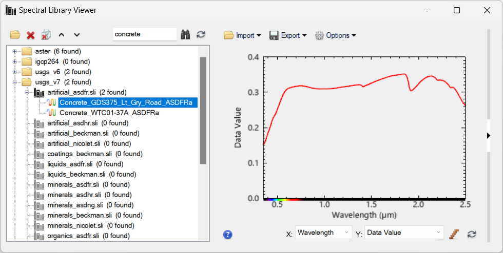
Figure 16 – Spectral signature for light gray road concrete material from USGS v7 library

Once an appropriate reference spectral signature has been identified for the material of interest the workflow can be executed against an atmospherically corrected hyperspectral imagery dataset.

1. Open and display the QUAC atmospheric correction output processing result raster dataset so the imagery data being analyzed has bottom-of-atmosphere (BOA) surface reflectance pixel units.
2. Within the Toolbox panel on the right-hand side of the ENVI software window type target detect string in the blank search text box, press the Enter key on the keyboard, and double-click on the Target Detection Workflow tool.
3. In the workflow Select Data step to the right of the blank Input Raster text box press the Browse… button, select the QUAC output raster dataset and press OK button, then press the Next >> button to proceed to the next step in the workflow.
4. In the workflow Select Signatures step make sure the Target subfolder list item is selected then press the Import button and from the drop-down list menu select From Spectral Library….
5. In the resulting Import from Spectral Library dialog within the top Library section list scroll down and select the usgs_v7\artificial_asdfr.sli spectral library file. Next, in the blank Search… text box to the right of Spectra label enter the text string concrete then select the Concrete_GDS375_Lt_Gry_Road_ASDFRa item in the list, press OK button to dismiss the pop-up dialog, then press the Next >> button to proceed to the next step in the workflow.
6. In the workflow Image Transform for Dimensionality Reduction step select Skip this step radio button then press the Next >> button to proceed to the next step in the workflow.
7. In the workflow Target Detection step click the Method drop-down list, select Spectral Angle Mapper Classification algorithm from the menu, then press the Next >> button to proceed to the next step in the workflow.
8. In the workflow Threshold step interactively drag the red threshold bar on the SAM classification histogram to an appropriate level aligned with peak spectral target detections then press the Next >> button to proceed to the next step in the workflow.
9. In the workflow Smooth step leave all parameters set to their default settings then press the Next >> button to proceed to the next step in the workflow.
10. In the workflow Export Final Result step specify output filenames for both the Export Classification Raster and Export Shapefile then press the Finish button to complete execution of the target detection workflow.

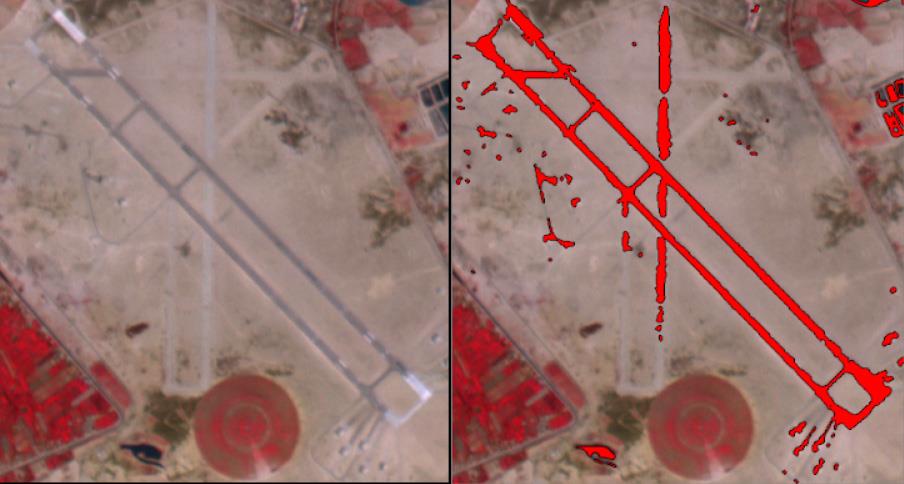
Figure 17 – CIR image (left) and spectral target detection of light gray road concrete (right)

Once the spectral target detection workflow is finished running the output classification raster and vector shapefile datasets can be displayed to illustrate the regions in the imagery where there is a high likelihood match to the spectral signature for light gray road concrete material from the reference spectral library.

Supervised Classification

The ENVI software includes a wide variety of advanced Classification Tools that can be used to perform a supervised classification of hyperspectral imagery datasets in order to generate a map of different land use land cover (LULC) types. The supervised classification process in the ENVI software is a multi-step workflow which involves the manual creation of supervised training data for the different class types, execution of a supervised classification algorithm, post-classification cleanup, and raster-to-vector conversion for processing result output to common GIS mapping formats such as Shapefile. The ENVI software provides a powerful Region of Interest (ROI) Tool for definition of supervised training data along with a convenient guided Classification Workflow that walks users through these multiple steps in order to generate GIS mapping layers.

1. Open and display the QUAC atmospheric correction output processing result raster dataset so the imagery data being analyzed has bottom-of-atmosphere (BOA) surface reflectance pixel units.
2. While the QUAC-processed imagery dataset is selected in the Layer Manager panel on the left-hand side of the ENVI software window launch the ROI Tool by selecting File -> New -> Region of Interest from the main menu or press the button on the toolbar at the top of the main ENVI software user interface window.
3. Within the Region of Interest (ROI) Tool pop-up dialog window press the button to initialize a new ROI and in the text box to the right of the ROI Name label change the name of the ROI #1 to a more suitable name for the training data class type being defined (e.g., Open Water).
4. Follow the instructions in the ENVI software documentation on how to utilize the Region of Interest (ROI) Tool in order to define separate ROI classes for each unique land use land cover (LULC) type in the geographic region where the atmospherically corrected hyperspectral imagery dataset is located.
5. One of the simplest ways to quickly and effectively create supervised training data ROIs for remote sensing imagery is to leverage the Create ROIs from Pixels functionality available when the Region of Interest (ROI) Tool dialog window is selected.
6. Repeat the process of creating a new ROI for every land use land cover (LULC) class type that should be classified using the supervised image classification workflow.
7. Once finished creating all of the desired ROIs save the training data to an XML format file on disk by selecting File -> Save As… from the Region of Interest (ROI) Tool dialog menu.

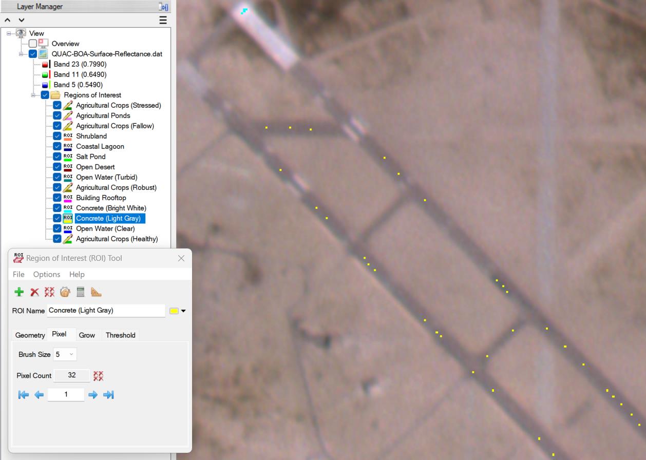
Figure 18 – The ENVI software Region of Interest (ROI) Tool being used to manually create separate supervised training data ROIs for distinct land use land cover (LULC) class types

Now that the ROI Tool has been used to generate supervised training data, the next step is to run the Classification Workflow.

1. Within the Toolbox panel on the right-hand side of the ENVI software window type classification workflow string in the blank search text box, press the Enter key on the keyboard, and double-click on the Classification Workflow tool.

2. In the workflow File Selection step make sure the QUAC output raster dataset is selected for the Input Raster File: field then press the Next > button to proceed to the next step in the workflow.

3. In the workflow Classification Type step select the Use Training Data radio button then press the Next > button to proceed to the next step in the workflow.

4. In the workflow Supervised Classification step the previously defined ROIs should be automatically loaded into the Training Data list panel (if not then press the Load Training Data Set button and load the ROIs previously saved to the XML format file on disk).

5. Select the Algorithm tab, click the drop-down list at the top of the tab panel, then select Spectral Angle Mapper algorithm.

6. In the lower left-hand corner of the Classification workflow dialog check the Preview checkbox then use the main image display navigation controls to move the underlying image around to view a preview of the SAM image classification result within the preview inlay box:

   

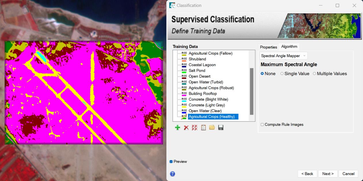
7. If necessary make advanced adjustments to the Maximum Spectral Angle by either specifying a Single Value threshold or set Multiple Values individually for each ROI class.

8. Once satisfied with the SAM image classification configurations press the Next > button to proceed to the next step in the workflow.

9. In the workflow Cleanup step leave all parameters in their default settings and press the Next > button to proceed to the next step in the workflow.

10. In the workflow Cleanup step specify output filenames for both the Export Classification Image and Export Classification Vectors then optionally export the classification statistics to a text file on disk.

11. Once finished specifying the output filenames press the Finish button to complete execution of the classification workflow.

Once the Classification Workflow processing steps have finished running the output classification raster and vectors will be automatically loaded into the active view display window where the land use land cover (LULC) classification results can be visualized.

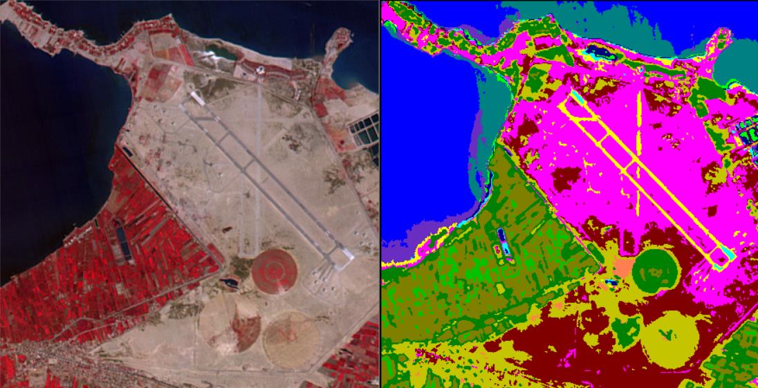
Figure 19 – CIR image (left) and supervised classification workflow processing results (right)