Hyperspectral signatures

Every pixel in a hyperspectral image has a spectrum: its reflectance in each band. That spectrum depends on what's in the pixel, and comparing it against known spectra is how you work out what the pixel contains. This page covers spectral signatures, the complication of mixed pixels, and the two broad ways of working with them.

Spectral signatures

A spectral signature is a material's reflectance plotted against wavelength. Signatures are usually measured in a laboratory or the field on a pure sample, and collections of them are called spectral libraries. See material reflectance libraries for where to find them.

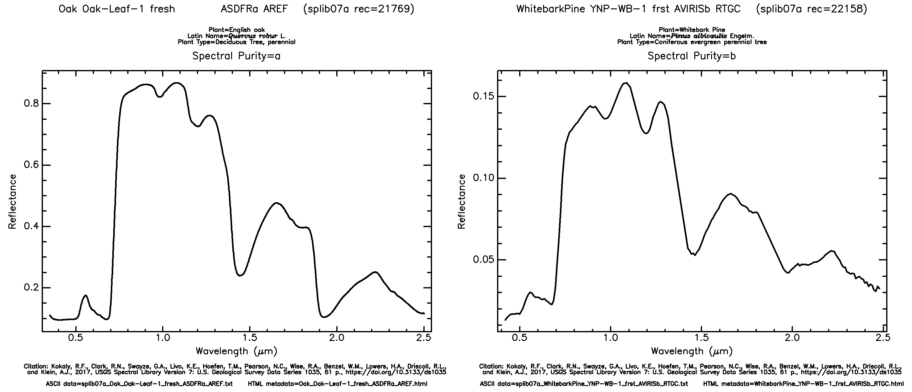
Signatures of whitebark pine and English oak from the USGS Spectral Library version 7. Both are vegetation and share the same overall shape; the differences between them are what a hyperspectral sensor can pick up and a multispectral one mostly can't.

Before you compare a library spectrum with a pixel, resample it to the sensor's bands. Library spectra are often sampled every 1 nm, while each Dragonette band averages over 15 to 32 nm, so the two only line up once the library spectrum has been averaged through each band's response. The rare earth elements tutorial shows how.

Mixed pixels

A pixel often contains more than one material, and its spectrum is then a blend of theirs, roughly in proportion to how much of the pixel each one covers. This is called a mixed pixel, and it means a pixel's spectrum won't match any single library signature exactly.

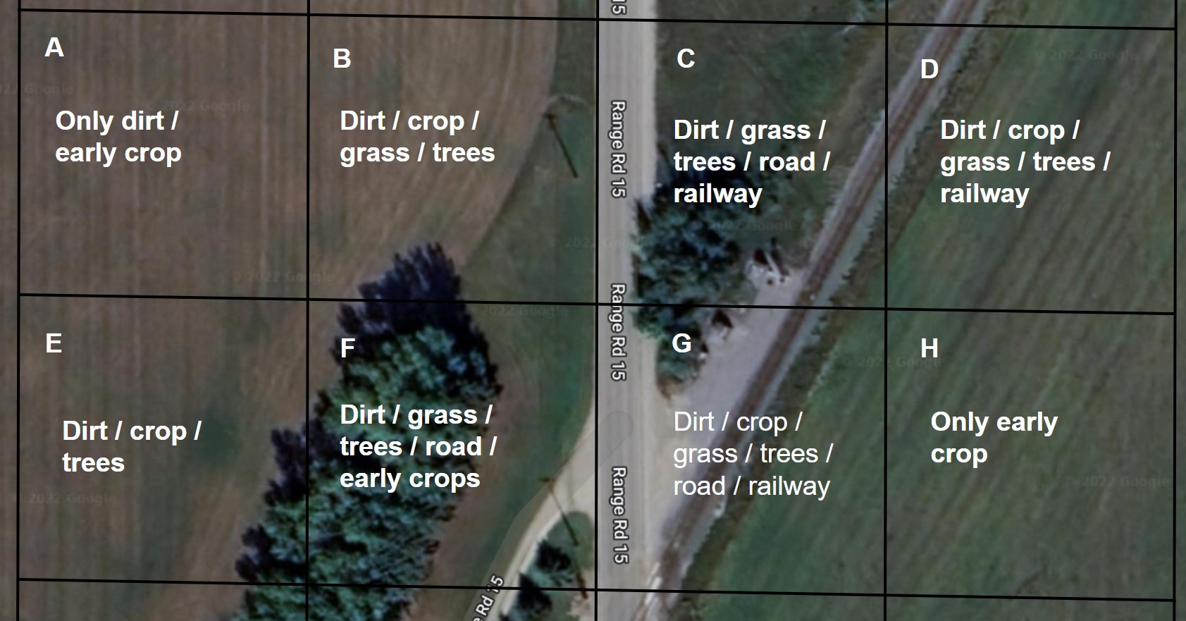
Coarse pixels (black boxes) over two fields. Pixels inside a field are pure; pixels over the road, railway, and field edges are mixed.

The coarser the pixel, the more of them are mixed, because each one covers more ground. At 5.3 m, a Dragonette pixel is small enough to fall inside a single field, roof, or stand of trees far more often than a 30 m pixel is, but mixing never goes away entirely. Field edges, roads, and small features will always produce mixed pixels.

There are two ways to deal with mixing: model it, or classify each pixel by its closest match.

Unmixing pixels

The first approach models the mixing directly. Endmember extraction finds the purest spectra in a scene, the endmembers, which represent its main materials. Spectral unmixing then estimates what fraction of each pixel is made up of each endmember, so instead of labelling a pixel "field" or "road" you get a map of how much of each it contains. Spectral Python (SPy) implements endmember extraction and documents how to apply it.

Classifying pixels

The second approach is to compare each pixel with known signatures and assign it to the closest match. Because library spectra are measured under laboratory conditions and image spectra aren't, you're looking for the most similar signature rather than an exact one. The spectral angle mapper (SAM) is the classic example. It compares the shape of two spectra and ignores their overall brightness, so a shaded pixel still matches a sunlit library spectrum of the same material. The rare earth elements tutorial uses a related detector, ACE, to find bastnaesite, a neodymium-bearing mineral, at the Mountain Pass mine in California.

Spectral Python also provides supervised classification algorithms.