Plant Health Indices

Background

Multi-spectral imagery from satellites like Landsat and Sentinel-2 have typically been used to calculate indices like NDVI, SAVI, and EVI. These indices enable us to measure the presence and general overall health of vegetation within a scene. Unfortunately, due to the width and number of bands within multi-spectral satellites, we are unable to quantify specific features of plant health like chlorophyll and carotenoid content or leaf area index.

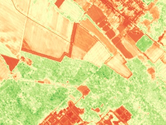
As we can see from the images below, NDVI is still capable of reliably separating vegetation from the surrounding scene. We can also see areas of denser plant growth, and can discern lines of crops within a field.

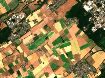
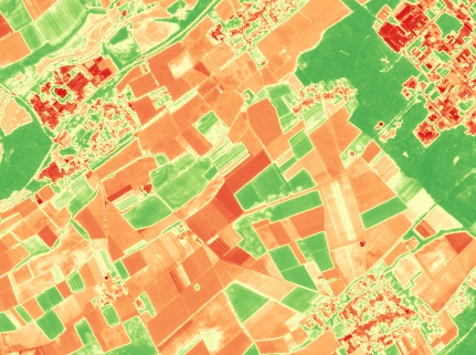
Sentinel-2 RGB

Sentinel-2 NDVI

Sentinel-2 RGB (true color) and calculated NDVI index

We can visualize the band width of typical multi-spectral satellites with the below image. We can see that the use of a near-infrared bands allows us to effectively isolate green vegetation from soil, as vegetation has a significantly different reflectance curve. We can also see that the band widths are quite wide. For example, Sentinel-2's Band 8 (NIR, #4 in this image) has a band width of approx. 100nm.

Figure 1: Wide bandwidths of multi-spectral satellites [4]

When we compare multi-spectral bandwidths to the below image of more detailed vegetation reflectance curves, we can see that plants actually have an incredible amount of information that would otherwise be undetectable with multi-spectral satellites. It's clear that hyperspectral sensors would be able to glean significantly more information about a plant's health than multi-spectral sensors.

Figure 2: Overview of crop stages & reflectance, with key areas highlighted [5]

Plant Health

Figure 3: Absorbance curves of plant compounds [1]

There are many aspects of plant health that we can quantify based on the reflectance of plant foliage.

• Chlorophyll: Green pigments that allow a plant to absorb energy from light.
• Carotenoids: Yellow, orange, and red pigments that have many functions within a plant. High levels of carotenoids with an absence of chlorophyll is indicative of plants that are not healthy.
• Anthocyanins: Purple, blue, or black pigments that are usually not present during the growing season. Anthocyanins are produced towards the end of summer, and are responsible (along with carotenoids) for the leaf colors we see in fall.
• Leaf Area Index (LAI): Dimensionless quantity that quantifies green leaf area in relation to ground surface area.
• Red Edge Position: Position of a rapid change in reflectance that occurs in the near-infrared range of light. Useful for crop identification, growth phase, crop monitoring, disturbance detection, and canopy stress.
• Senescence: The process of aging in plants. Usually tied to an increase in anthocyanins (in annuals & perennials) and a decrease in chlorophyll.

There are many different combinations of hyperspectral & multi-spectral bands that can be used to quantify these aspects of plant health. Below are a selection of popular indices, and their applicability to certain satellites.

note

This is just a small selection of indices! Longer lists are available from sources at the bottom of this article!

Index	Applications	Sentinel‑2	Landsat 7/8	SuperDove	Wyvern Dragonnette	Wyvern Gen 2
NDVI	General plant health & presence of vegetation				*	*
EVI	General plant health & presence of vegetation, counteracts NDVI saturation problem				*	*
SAVI	General plant health & presence of vegetation, suppresses effect of soil pixels				*	*
RENDVI	Sensitive to small changes in senescence & foliage content
VREI2	Sensitive to chlorophyll concentration, leaf area index, and water content
REPI	Crop identification, disturbance detection, canopy stress
ARI1/2	Sensitive to weakening vegetation due to high concentration of anthocyanins
CRI1/2	Sensitive to stressed vegetation due to high concentration of carotenoids
SIPI/1	Sensitive to ratio of carotenoids to chlorophyll
NDWI	Sensitive to changes in canopy water content
CAI	Sensitive to cellulose, useful in fire fuel conditions and crop residue monitoring

info

Since hyperspectral imagery has narrower bandwidths, broadband indices can be replicated by combining multiple narrow bands or selecting a similar narrowband index.

Hyperspectral Indices

note

There are an incredible amount of hyperspectral indices available. With many applications including assessing plant health, urban environments, and measuring the prescence of water & snow. We will only highlight some of the most popular hyperspectral indices here, however additional resources are listed at the bottom of this article and are worth looking into!

RENDVI (Red Edge Normalized Difference Vegetation Index)

RENDVI is the narrowband equivalent of NDVI. This index takes advantage of slight changes in sensitivity of vegetation in the red edge band (750 nm) to examine changes in foliage and senescence. RENDVI also has the advantage of not "saturating" to the extent that NDVI does (see below, some areas of plant growth in the Sentinel-2 NDVI are completely green).

Sentinel-2 NDVI

Wyvern RENDVI

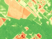
Comparison of 10m Sentinel-2 NDVI to 5m Wyvern RENDVI

We are also putting the Sentinel-2 imagery at a distinct disadvantage here, as the resolution (Ground Sampling Distance) is 10m compared to Wyvern Dragonette's 5m GSD. That being said, it's clear that RENDVI provides clear benefits to the traditional broadband NDVI.

VREI2 (Vogelmann Red Edge Index 2)

VREI2 is a narrowband index that is effective in light or dark backgrounds [2]. It is sensitive to the combined effects of foliage cholorphyll concentration, leaf area index, and water content [3].

Wyvern RENDVI

Wyvern VREI2

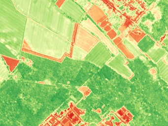
Comparison of 5m Wyvern RENDVI to 5m Wyvern VREI2

When comparing RENDVI to VREI2 in the above image, a number of things can be discerned. The field in the top-right is significantly greener than other fields when viewed in the VREI2 index. This field is growing maize, whereas fields in the left of the image are growing wheat and sugar beets (according to the EU 2018 crop map). Areas of more vigourous growth can also be identified in the forest at the bottom of the image in VREI2.

Do it Yourself!

Below is an example of how to calculate RENDVI from a hyperspectral image. It requires you to setup a python environment with Numpy, Rasterio, and Matplotlib. We highly recommend you use Anaconda to install these packages (Rasterio relies on GDAL which is notorious for being hard to install). Once you run this code, you should have an output that looks like the following:

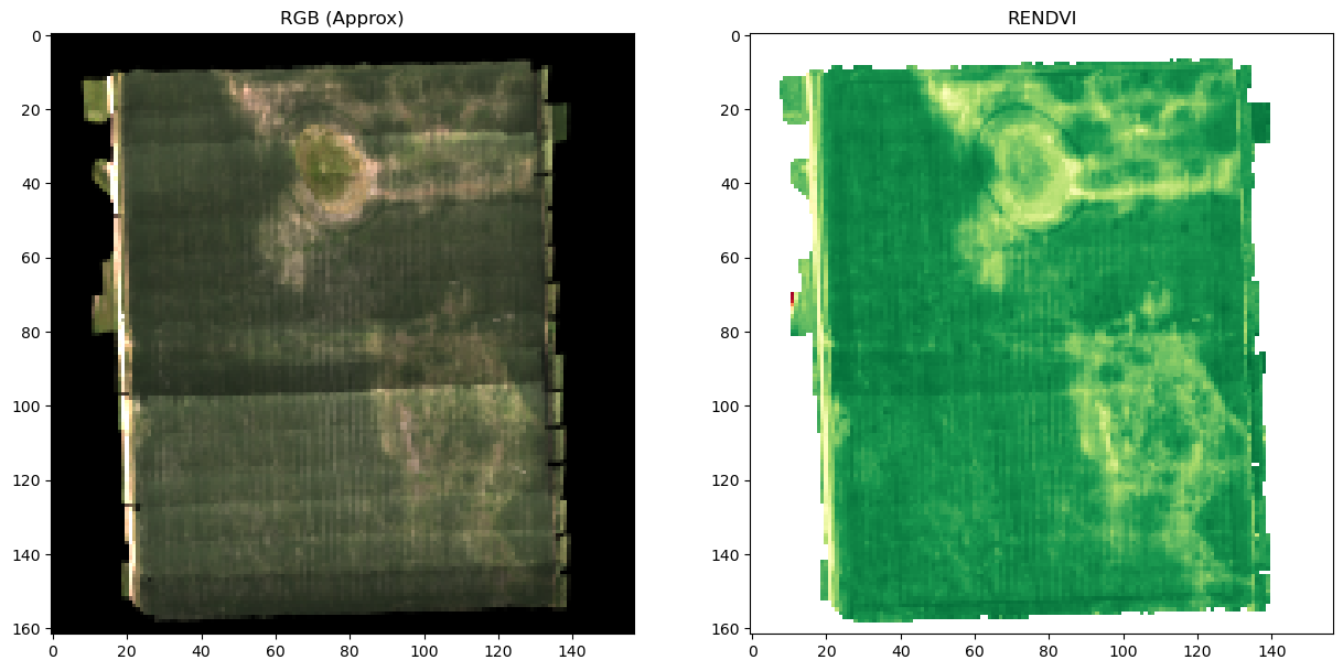
RGB & RENDVI Output

import rasterio

import numpy as np
import matplotlib.pyplot as plt


# We're using GDAL's vsis3 driver to read from a public S3 URL.  You can change this to wherever your copy
# of the data is stored.
INPUT_FILE_PATH = "/vsis3/wyvern-drone-data-processed/processed/SFB1516/WYVERN_SFB1516_20220726_v0_1_0_5mGSD.tiff"
OUTPUT_FILE_PATH = "rendvi_output.png"

# First, let's read our hyperspectral image using rasterio
image = rasterio.open(INPUT_FILE_PATH)
image_arr = image.read()

# Indicies 23 & 19 correspond to the closest bands to the RENDVI formula. (750.179nm & 701.382nm)
# Band wavelengths can be accessed by calling `image.descriptions`
band_750nm = image_arr[23]
band_705nm = image_arr[19]

# We'll also grab a pseudo-RGB array we can plot alongside the RENDVI!
# These are array indices that are close to red, green, and blue channels we would see with our eyes.
rgb_array = image_arr[[12, 6, 1]]
rgb_array = np.moveaxis(rgb_array, 0, -1)  # Move axis just puts our RGB channel at the end of the array

# Now we can use the RENDVI formula to calculate the index
# 750nm - 705nm / 750nm + 705nm
rendvi_array = (band_750nm - band_705nm) / (band_750nm + band_705nm)

# We can now plot the array using matplotlib!
fig, axs = plt.subplots(1, 2, figsize=(15, 10))
axs[0].imshow(rgb_array * 9)  # Quick way to increase brightness
axs[1].imshow(rendvi_array, cmap="RdYlGn")

axs[0].set_title('RGB (Approx)')
axs[1].set_title('RENDVI')

# And now we can export as an image!
plt.savefig(OUTPUT_FILE_PATH)

More Resources

Check out our deep dive into hyperspectal indices at our Index Library!

Citations

[1] Zhou, Ning & Dong, Weiming & Mei, Xing. (2006). Realistic Simulation of Seasonal Variant Maples. 295 - 301. 10.1109/PMA.2006.29.

[2] Vogelmann, Jim & Rock, Barrett & Moss, D.M.. (1993). Red edge spectral measurements from sugar maple leaves. Int. J. Remote Sens.. 14. 10.1080/01431169308953986.

[3] Velichkova, Kalinka & Krezhova, Dora. (2019). COMPARATIVE ANALYSIS OF HYPERSPECTRAL VEGETATION INDICES FOR REMOTE ESTIMATION OF LEAF CHLOROPHYLL CONTENT AND PLANT STATUS. RAD Association Journal. 3. 10.21175/RadJ.2018.03.034.

[4] Pham, Binh. (2018). Satellite remote sensing of the variability of the continental hydrology cycle in the lower Mekong basin over the last two decades. 10.13140/RG.2.2.27136.07686.

[5] Hyperspectral Signatures by USGS Western Geographic Science Center